Static vs. Dynamic vs. Continuous Batching in LLMs, clearly explained

Everything you need to understand why your GPU sits idle under load and which batching strategy fixes it. Three strategies from first principles, the flaw each one leaves behind, chunked prefill, and how to choose for your workload.
A modern GPU can run trillions of floating-point operations every second. Serving an LLM on one, you will often watch it sit at a small fraction of that.
The reason is that generating a single token means reading every weight in the model out of memory. That read dominates the time, and the compute units spend most of it waiting.
Batching closes the gap. Load the weights once, push many sequences through the same pass, and the memory cost gets spread across all of them.
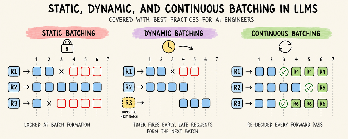
Every serving engine does this. What separates them is when the batch gets decided.
That last one is where nearly all the throughput in modern serving comes from. The other two are worth understanding first, since each fails in a way the next is built to fix.
And today we are going to break down and understand each of them one by one.
Let's go! 🚀
Why batching exists
An A100 does roughly 312 teraFLOPs of BF16 math per second and moves about 2 terabytes per second out of memory. Decoding leans entirely on the second number.
Reading the weights is the whole cost, and the compute sits idle waiting. That idle compute is free capacity, so a batch of sixty rides the same weight read as the batch of one did, and throughput climbs while the memory read time stays the same.

Note that, throughput climbs steeply with batch size, then flattens.
The bend moves with the model, the GPU, and the sequence length, so measure it on your own hardware.

Now, you might be thinking: if batching is this effective, why not batch as much as possible?
Well, with LLMs, that is harder than it sounds. Let’s understand why.
What breaks for LLMs
Batching is older than LLMs. For a classifier or an embedding model, it is a packing problem.
Pad the inputs to a common length, stack them into one tensor, run one pass.
That works because three things hold. One pass produces the whole answer, no row depends on another, and every row's cost is known before it starts.
This doesn't work for autoregressive LLMs.
Decoding breaks all three.

Padding does not rescue this. It equalizes input width, not how long a request holds the GPU.

So a batch fixed at the start runs at the pace of its slowest member. The three strategies are three answers to that, in increasing order of how much they do about it.
Static batching
The simplest answer does nothing about it. Collect a fixed number of requests, run them together, and return everything when the last one finishes.
Here's how the end state looks like:

R3 stops generating at t=9 and sits on the GPU until t=15, because R2 is still running. That costs you twice:
Waste scales with higher output variance. Anyscale measured this on OPT-13B on a 40GB A100. Widening the spread of output lengths dropped static batching to roughly 81 tokens per second, while continuous batching held an order of magnitude higher.

Still the right call sometimes. Static batching only looks bad when output lengths vary. Take that away and the slow-member problem goes with it.
Classification, embeddings, and scoring do exactly that. Each emits a fixed-size output, a label or a vector, so every request in the batch finishes at nearly the same step and none waits on a straggler.
For that kind of work, static batching is simpler and gives up nothing.
Here's how you configure static batching in vLLM:
from vllm import LLM, SamplingParams

llm = LLM(model="meta-llama/Llama-3.1-8B-Instruct")
outputs = llm.generate(prompts, SamplingParams(max_tokens=64))
llm.generate hands the engine the whole workload at once. Cap max_tokens, keep prompt sizes similar, and every sequence finishes at nearly the same step.
👉 The Hugging Face pipeline API with a batch_size argument is also static batching. Fine for evaluation scripts, poor for live traffic.
Dynamic batching
Static batching has a second cost. A request can wait a long time just to enter a batch.
If the batch size is 8 and only 5 have arrived, those 5 sit idle until three more show up.
Dynamic batching adds a timer. The batch fires on the size limit or when the window expires, whichever comes first.
Here's how the end state looks like:

Batch 1 fires at t=4 (the fixed interval) with only R1 and R2, because the window expired before a third arrived. Both start four units earlier than static batching allowed.
It shortens the wrong wait. R1 finishes at t=7 and still waits until t=12, because R2 is not done.
Dynamic batching decides once per batch, then hands control to the engine until every member is done. For fixed-output models that is a complete answer, which is why Triton ships it.
dynamic_batching {
  preferred_batch_size: [ 4, 8 ]
  max_queue_delay_microseconds: 100
}
👉 preferred_batch_size lists the sizes the scheduler tries to form. max_queue_delay_microseconds caps how long a request waits for company.
Continuous batching
Both strategies so far treat a batch as one unit of work that starts and runs until every request in the batch has finished. That assumption is what still costs you, and continuous batching drops it.
The scheduler runs one iteration, gets control back, and decides again. The moment a sequence emits its final token it leaves the batch, and a waiting request takes that slot on the next pass.
The batch composition changes every iteration, which is why this is iteration-level scheduling. No slot waits for the slowest sequence, so the GPU stays saturated even when output lengths vary wildly.
This is how the end state looks liek:

The limit is memory, not compute. Every active sequence holds a KV cache that grows with each token, and that cache, not the math, is what caps how many sequences fit.
On a 40GB A100 with a 13B model resident, only a handful of long sequences fit at once. When the pool runs out, the scheduler evicts a running request and recomputes it later.
That looks like the GPU running out of headroom, when it is really the same prefill computed twice.
👉 Every engine ships continuous batching under a different name: vLLM, SGLang, and TGI call it that, TensorRT-LLM calls it in-flight batching, LMDeploy calls it persistent batching.
Chunked prefill
Rebuilding the batch every pass fixes the slow-member problem and introduces a new one, which users see as a stutter.
A joining request is prefilled in one iteration. A 32K-token prompt is one large, compute-heavy pass that every active decode waits behind, so output pauses mid-sentence because someone else pasted a long document.
Here's how things look without and with chunked prefill.
Whole prefill:

Chunked prefill:
(prompt of request C is broken down into smaller chunks of 2k tokens each)

Split the prompt across iterations. Chunked prefill breaks the prompt into fixed-size token ranges scheduled over several passes, each extending the request's KV cache.
The attention math is unchanged, since later chunks attend to what earlier chunks processed. The first token arrives after the final chunk.
Prefill is compute bound and decode is memory bound, so one batch containing both uses both parts of the chip.

When choosing values, note that:
Chunked prefill is on by default in vLLM V1, where --max-num-batched-tokens caps tokens per iteration. SGLang uses --chunked-prefill-size, and -1 disables it.
vLLM:
vllm serve meta-llama/Llama-3.1-8B-Instruct \
  --max-num-batched-tokens 8192
SGLang:
sglang serve --model-path meta-llama/Llama-3.1-8B-Instruct \
  --chunked-prefill-size 8192
👉 There is no universal best chunk size. It depends on the model, the GPU, your prompt length distribution, and which latency metric your SLO measures.
Conclusion
The three strategies differ only in when they fix the batch, and each answers a different workload shape.
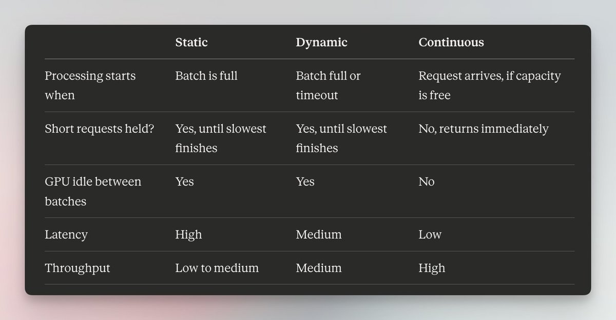
For live traffic with variable output lengths, continuous batching is the only one that holds up, and every major engine gives it to you by default.
This whole article rests on one fact about GPUs: a forward pass is bottlenecked on reading weights out of memory, not on the math.
I have written a detailed article on how a GPU works:
It builds up from first principles why memory and compute compete, why that gap exists in the hardware, and what makes a workload memory-bound in the first place. It needs no prior background, and it is the natural prequel to everything above.
Stay tuned for more!
Thanks for reading.
Cheers! :)
