Team sport sprint profiling for dummies “Speed kills” but faulty...

Eamonn Flanagan@EamonnFlanagan
35 views
Dec 20, 2024
~3 min read
Advertisement
1
Team sport sprint profiling for dummies
“Speed kills” but faulty interpretation of speed data, kills our ability to meaningfully assess sprint performance
Here's a super simple way to get more granularity from speed data 👇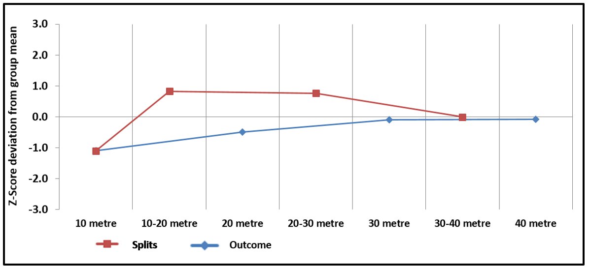
“Speed kills” but faulty interpretation of speed data, kills our ability to meaningfully assess sprint performance
Here's a super simple way to get more granularity from speed data 👇
2
In team sports, speed assessment involves testing athletes over 40m and analyzing their times at intervals (10/20/30/40).
Typically:
10m times are seen as markers of acceleration
40m times indicate top speed
Typically:
10m times are seen as markers of acceleration
40m times indicate top speed
3
Athletes are often ranked based on these times, either compared to teammates or against normative data.
While rankings might identify the fastest sprinters, they fail to show how an athlete achieves their performance.... or where improvement opportunities lie.
While rankings might identify the fastest sprinters, they fail to show how an athlete achieves their performance.... or where improvement opportunities lie.
4
Rankings are DECEPTIVE:
A tiny gap (e.g., 0.01s) between 1st and 2nd might look significant but isn't meaningful.
A larger difference (e.g., 0.1s) between 2nd and 3rd may reflect a much bigger performance gap.
Often rankings or absolute outcomes drive narratives
A tiny gap (e.g., 0.01s) between 1st and 2nd might look significant but isn't meaningful.
A larger difference (e.g., 0.1s) between 2nd and 3rd may reflect a much bigger performance gap.
Often rankings or absolute outcomes drive narratives
5
Team sport athletes often display distinct sprint profiles:
An athlete may excel in early acceleration (0–10m) but struggle to accelerate longer
Another might have poor initial acceleration yet accelerate longer and hit high maxV later (30–40m)
An athlete may excel in early acceleration (0–10m) but struggle to accelerate longer
Another might have poor initial acceleration yet accelerate longer and hit high maxV later (30–40m)
6
Both athletes could end up with an “average” 40m time, yet their training needs differ dramatically.
Splits combined with outcomes provide clarity: they highlight strengths and weaknesses across different phases of the sprint.
Splits combined with outcomes provide clarity: they highlight strengths and weaknesses across different phases of the sprint.
7
Solution: Use z-scores to contextualize an athlete’s split performance against their peers.
A z-score for each split (not outcome) shows how far a result deviates from the group mean:
A positive z-score = better than average.
A negative z-score = below average.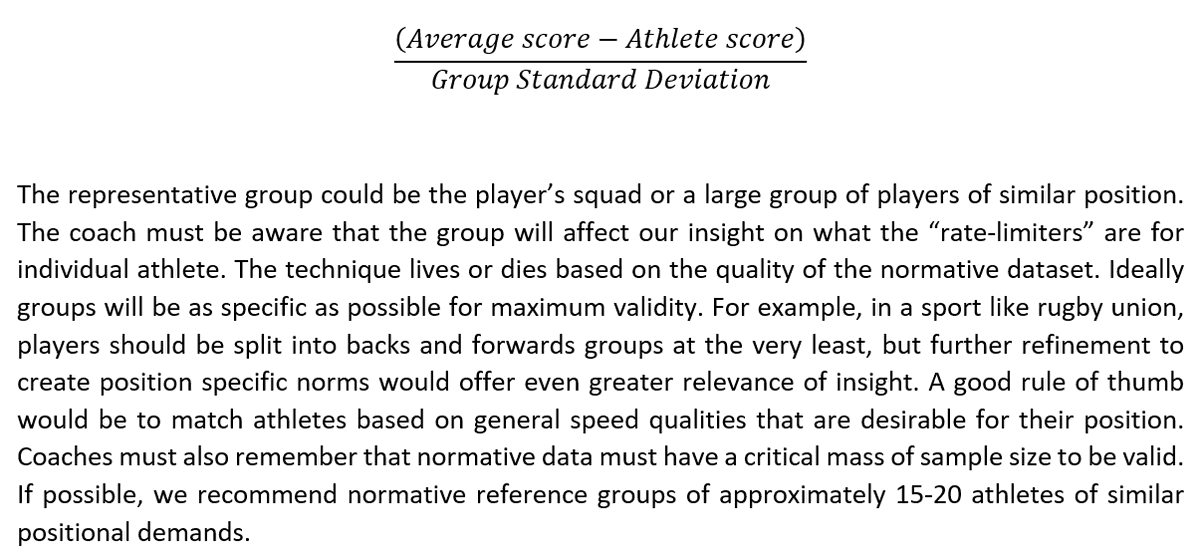
A z-score for each split (not outcome) shows how far a result deviates from the group mean:
A positive z-score = better than average.
A negative z-score = below average.
8
[Technical note:]
When applied to sprints, "flip" z-scores: faster times get higher z-scores, "better than average".... making visualizations intuitive—higher scores mean better speed.
When applied to sprints, "flip" z-scores: faster times get higher z-scores, "better than average".... making visualizations intuitive—higher scores mean better speed.
9
How It Works
Collect group or historical data (squad or position-specific peers)
Calculate mean & StDev for:
Outcomes (10/20/30/40)
Splits (0–10/10–20/20–30/30–40)
Convert each athlete’s performance into z-scores, creating a more detailed profile from the SAME dataset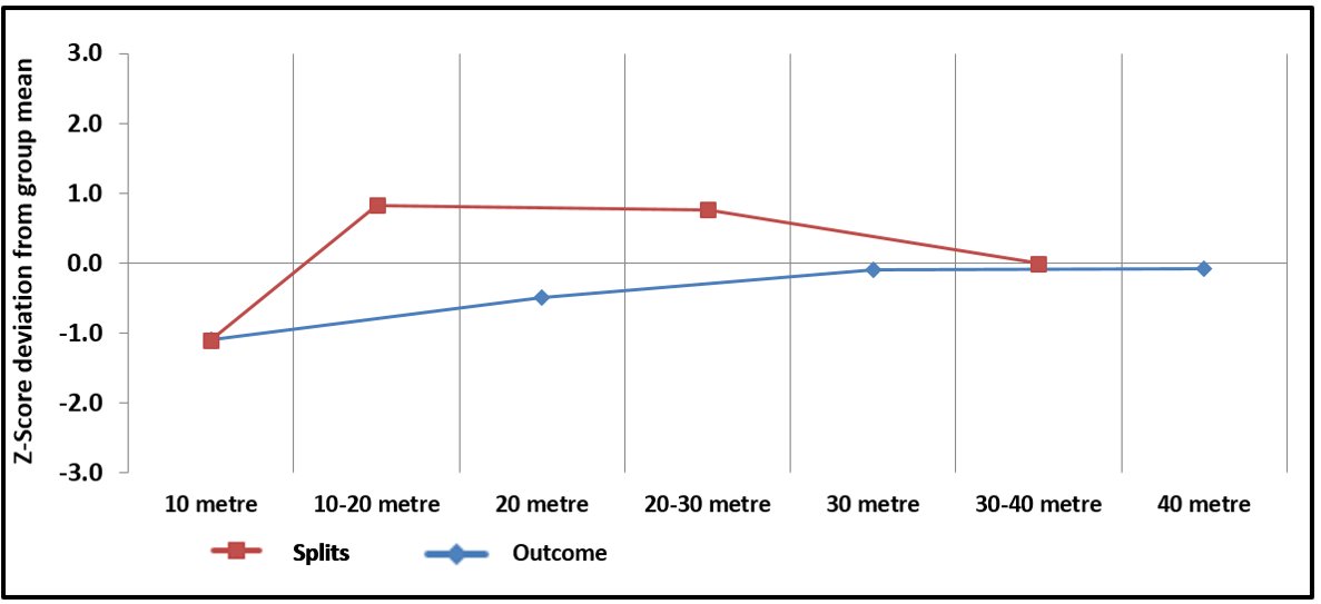
Collect group or historical data (squad or position-specific peers)
Calculate mean & StDev for:
Outcomes (10/20/30/40)
Splits (0–10/10–20/20–30/30–40)
Convert each athlete’s performance into z-scores, creating a more detailed profile from the SAME dataset
10
Split profiles provide a clearer understanding of athletes' abilities:
Positive: Performance improves across the sprint.
Negative: Strong start but struggles to sustain acceleration.
Deficit Profile: A clear weak phase (e.g., poor 20–30m performance).
Neutral Profile: Consistent across phases.
Positive: Performance improves across the sprint.
Negative: Strong start but struggles to sustain acceleration.
Deficit Profile: A clear weak phase (e.g., poor 20–30m performance).
Neutral Profile: Consistent across phases.
11
Below is example profile, a typical “deficit” profile.
The coach can qualitatively assess the plot and identify any noticeable deficits.
For these “deficits”, the absolute differences from the average can be examined in real terms (time difference from the group mean).
On inspection of absolute time differences we can make a more informed decision on whether or not the identified “deficit” is meaningful to performance or not.
The method is a first step to identifying deficits and additional performance testing data can be used to investigate further.
The coach can qualitatively assess the plot and identify any noticeable deficits.
For these “deficits”, the absolute differences from the average can be examined in real terms (time difference from the group mean).
On inspection of absolute time differences we can make a more informed decision on whether or not the identified “deficit” is meaningful to performance or not.
The method is a first step to identifying deficits and additional performance testing data can be used to investigate further.
12
Enhance overall profiling w/ relevant strength quality assessments for more holistic insights
Example: A team sport athlete w/ long contact times (via RSI testing) may benefit from short-contact plyometrics & ankle-dominant work to improve late-phase acceleration
Example: A team sport athlete w/ long contact times (via RSI testing) may benefit from short-contact plyometrics & ankle-dominant work to improve late-phase acceleration
13
Use split based profiling to uncover strategies behind the team sport athletes sprint performance
Strategy > Outcome
Different profiles demand different interventions: tailor interventions
Sprint variability profiling uses the data you already have, leverage it
Strategy > Outcome
Different profiles demand different interventions: tailor interventions
Sprint variability profiling uses the data you already have, leverage it