As we scale to trillion parameter models and gigawatt-scale...

Aarav Wattal@aaravwattal
25 views
Aug 23, 2026
~7 min read
Advertisement
1
As we scale to trillion parameter models and gigawatt-scale training, we don't do interesting work on just one chip anymore. Everything interesting happens across thousands of them, and moving data between those chips has become a fundamental bottleneck of both training and inference.
I spent this summer working on NVIDIA Feynman chip-to-chip interconnect, and wanted to share some things I've learned about the communication stack 🧵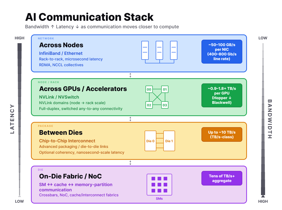
I spent this summer working on NVIDIA Feynman chip-to-chip interconnect, and wanted to share some things I've learned about the communication stack 🧵
2
The first thing worth internalizing is that "communication" isn't one thing, it's a hierarchy, and each tier costs each tier out costs several times more than the one inside it.
Two compute units on the same die talk at tens of TB/s. Two dies in the same package get 10 TB/s on Blackwell's die-to-die link. Two GPUs in a rack over NVLink 5 get 1.8 TB/s (bi-directional), and NVLink 6 doubles that to 3.6. Two GPUs in different racks over InfiniBand XDR get 800 Gb/s per NIC, which is 0.1 TB/s (more than an order of magnitude down).
The rule of thumb is the same one you know from the memory hierarchy: the further the data has to travel, the more you pay for it, in both latency and energy.
Two compute units on the same die talk at tens of TB/s. Two dies in the same package get 10 TB/s on Blackwell's die-to-die link. Two GPUs in a rack over NVLink 5 get 1.8 TB/s (bi-directional), and NVLink 6 doubles that to 3.6. Two GPUs in different racks over InfiniBand XDR get 800 Gb/s per NIC, which is 0.1 TB/s (more than an order of magnitude down).
The rule of thumb is the same one you know from the memory hierarchy: the further the data has to travel, the more you pay for it, in both latency and energy.
3
Adding more compute only helps if the rest of the system can keep up. At first glance scaling looks like a simple problem: if we double our compute, we should get a 2x speedup. But this falls apart as soon as synchronization enters the picture.
Let's say a training step is 100us of compute and 50us of allreduce/gradient sync, 150us total. If we quadruple the chip speed, compute drops to 25us but sync stays at 50us, so we paid for 4x and got 2x. Run the same experiment with a 16x faster chip and you land at 56us, barely better than the 4x chip, because at that point you're almost entirely paying for sync.
And that's the generous version, since it assumes sync doesn't get worse as you scale. In reality it does. Congestion, coordination overhead, and sometimes hop count tend to increase as the system scales, so the speedup curve doesn't just plateau, it can bend the wrong way.
Let's say a training step is 100us of compute and 50us of allreduce/gradient sync, 150us total. If we quadruple the chip speed, compute drops to 25us but sync stays at 50us, so we paid for 4x and got 2x. Run the same experiment with a 16x faster chip and you land at 56us, barely better than the 4x chip, because at that point you're almost entirely paying for sync.
And that's the generous version, since it assumes sync doesn't get worse as you scale. In reality it does. Congestion, coordination overhead, and sometimes hop count tend to increase as the system scales, so the speedup curve doesn't just plateau, it can bend the wrong way.
4
Training or serving a language model requires many different data communication patterns as we distribute it, and which pattern you're using decides which tier of the hardware stack it can afford to live on.
Tensor parallelism (TP) syncs every single layer, so it has to stay on the fastest fabric available (NVLink/NVSwitch inside a rack). Data parallelism (DP) syncs gradients during the backward pass (often bucketed and overlapped with compute), so it can tolerate the much slower fabric between racks. Pipeline parallelism (PP) splits the model by layer across chips and trades bandwidth for idle time (bubbles) while stages wait on each other, which makes it cheap on the wire but expensive in utilization.
Expert parallelism (EP) is the interesting one. It splits MoE experts across chips and needs all-to-all communication, but the traffic pattern is data-dependent on routing decisions made at runtime. So unlike the other three, it can be harder to overlap efficiently because routing is data-dependent, creating irregular all-to-all traffic and load imbalance.
Tensor parallelism (TP) syncs every single layer, so it has to stay on the fastest fabric available (NVLink/NVSwitch inside a rack). Data parallelism (DP) syncs gradients during the backward pass (often bucketed and overlapped with compute), so it can tolerate the much slower fabric between racks. Pipeline parallelism (PP) splits the model by layer across chips and trades bandwidth for idle time (bubbles) while stages wait on each other, which makes it cheap on the wire but expensive in utilization.
Expert parallelism (EP) is the interesting one. It splits MoE experts across chips and needs all-to-all communication, but the traffic pattern is data-dependent on routing decisions made at runtime. So unlike the other three, it can be harder to overlap efficiently because routing is data-dependent, creating irregular all-to-all traffic and load imbalance.
5
But it only takes one slow chip to stall an entire cluster. A sync point only completes when its slowest participant does, so what you pay is the max across all participants, not the average. And the more participants there are, the further out that max lands.
This is worth putting numbers on, because the intuition is easy to get wrong. With 8 independent chips, the median slowest chip lands around the 92nd percentile of the latency distribution (already in the tail), not the middle. Go to 1,000 chips and the median slowest chip is around p99.9. You didn't change any hardware you just drew more samples, and the worst of them got worse.
This is why step time at scale tracks tail latency rather than the mean, and why doubling cluster size can slow down every step on identical hardware. It's also part of why you never see spec-sheet bandwidth in practice - it’s a peak number, but real bandwidth is lower because the system adds overhead.
This is worth putting numbers on, because the intuition is easy to get wrong. With 8 independent chips, the median slowest chip lands around the 92nd percentile of the latency distribution (already in the tail), not the middle. Go to 1,000 chips and the median slowest chip is around p99.9. You didn't change any hardware you just drew more samples, and the worst of them got worse.
This is why step time at scale tracks tail latency rather than the mean, and why doubling cluster size can slow down every step on identical hardware. It's also part of why you never see spec-sheet bandwidth in practice - it’s a peak number, but real bandwidth is lower because the system adds overhead.
6
There's also a hard constraint underneath all of this that you can't buy your way past. With pairwise reduction, reducing N values down to 1 requires at least log(N) sequential combining rounds under any parallelization, because each round can at best halve the number of partial results you're still carrying. So if you have 16 chips and each round costs 10us, you're capped at 40us no matter how much bandwidth you throw at it. This is a latency problem.
But if a step can combine k inputs at once, the depth is closer to log_k(N), which is exactly why in-network reduction is interesting - the switch does the combining, and it can take more than two inputs at a time. You're not routing around the dependency chain, you're making it shorter.
It's also worth separating reduce from allreduce, since people use them interchangeably. A tree reduce gets the result onto one rank. If every rank needs it, you still have to broadcast it back out, which takes about another log(N) stages. Recursive-doubling allreduce can do the whole thing in about log(N) exchanges because every rank accumulates the result along the way.
Ring allreduce makes a different tradeoff. It takes about 2(N−1) steps, so latency grows with cluster size, but it uses bandwidth very efficiently. So trees tend to be better for small messages, while rings tend to be better for large ones. In practice, NCCL has several other algorithms too, and it picks based on the message size and how the GPUs are connected.
But if a step can combine k inputs at once, the depth is closer to log_k(N), which is exactly why in-network reduction is interesting - the switch does the combining, and it can take more than two inputs at a time. You're not routing around the dependency chain, you're making it shorter.
It's also worth separating reduce from allreduce, since people use them interchangeably. A tree reduce gets the result onto one rank. If every rank needs it, you still have to broadcast it back out, which takes about another log(N) stages. Recursive-doubling allreduce can do the whole thing in about log(N) exchanges because every rank accumulates the result along the way.
Ring allreduce makes a different tradeoff. It takes about 2(N−1) steps, so latency grows with cluster size, but it uses bandwidth very efficiently. So trees tend to be better for small messages, while rings tend to be better for large ones. In practice, NCCL has several other algorithms too, and it picks based on the message size and how the GPUs are connected.
7
And because everything in systems eventually comes back to roofline models, apply the roofline model to the network instead of HBM and you get what you might call a network ridge point: the minimum arithmetic intensity you need to stay compute-bound at the system level rather than the chip level.
It's just peak compute divided by fabric bandwidth, so it slides right whenever compute grows faster than the wires feeding it. The numbers are a little more nuanced though. NVLink went 600 GB/s on A100 to 900 on H100 (only 1.5x) then doubled on Blackwell and doubled again on Rubin. Interconnect is doing fine. And within a package, data doesn't have to leave around the chip's edge anymore. With microbumps and hybrid bonding, I/O can go through the face of the die instead.
So the ridge point still moves, just for a different reason. Most of the FLOP gain each generation comes from smaller number formats, and FP4 only helps if the tensors crossing the fabric shrink too. This often isn’t the case and tensor-core math may run at FP4 while gradients or activations stay at higher precision. So compute FLOPs can rise much faster than bytes on the wire fall.
It's just peak compute divided by fabric bandwidth, so it slides right whenever compute grows faster than the wires feeding it. The numbers are a little more nuanced though. NVLink went 600 GB/s on A100 to 900 on H100 (only 1.5x) then doubled on Blackwell and doubled again on Rubin. Interconnect is doing fine. And within a package, data doesn't have to leave around the chip's edge anymore. With microbumps and hybrid bonding, I/O can go through the face of the die instead.
So the ridge point still moves, just for a different reason. Most of the FLOP gain each generation comes from smaller number formats, and FP4 only helps if the tensors crossing the fabric shrink too. This often isn’t the case and tensor-core math may run at FP4 while gradients or activations stay at higher precision. So compute FLOPs can rise much faster than bytes on the wire fall.
8
The thing that surprised me is that copper is currently winning the short-distance fight. The NVLink spine inside an NVL72 rack is 5,184 copper cables, and the reason is power: doing that same link in optics would have burned around 20 kilowatts on transceivers before any compute happened. Over a meter, copper is still cheaper per bit.
Optics showed up first where the distances are longer, in the switches that connect racks to each other. So the real question isn't copper or optics, it's where the crossover sits - and every jump in data rate drags it closer.
At gigawatt scale, the interconnect ends up being just as big a design constraint as the compute itself on what models are actually trainable. Photonics changes this question from the ground up, but that's a post for another day.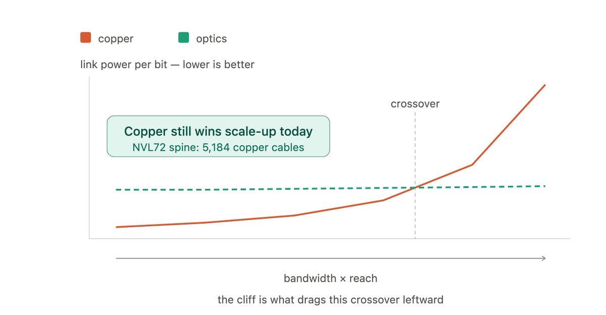
Optics showed up first where the distances are longer, in the switches that connect racks to each other. So the real question isn't copper or optics, it's where the crossover sits - and every jump in data rate drags it closer.
At gigawatt scale, the interconnect ends up being just as big a design constraint as the compute itself on what models are actually trainable. Photonics changes this question from the ground up, but that's a post for another day.
9
Thanks for reading and hope this was insightful! Feel free to reach out with any questions or thoughts - always happy to chat. And shoutout @AryaTschand for the thoughtful feedback 🙏
