Logistic Regression clearly explained 👇🏻

Josep Ferrer@iamjosepferrer
23 views
Feb 12, 2025
~2 min read
Advertisement
1
Logistic Regression clearly explained 👇🏻

2
1️⃣ 𝗟𝗢𝗚𝗜𝗦𝗧𝗜𝗖 𝗥𝗘𝗚𝗥𝗘𝗦𝗦𝗜𝗢𝗡
It is a binary classification model used to classify our input data into two main categories.
It can be extended to multiple classifications... but today we'll focus on a binary one.
Also known as Simple Logistic Regression.
It is a binary classification model used to classify our input data into two main categories.
It can be extended to multiple classifications... but today we'll focus on a binary one.
Also known as Simple Logistic Regression.
3
2️⃣ 𝗛𝗢𝗪 𝗧𝗢 𝗖𝗢𝗠𝗣𝗨𝗧𝗘 𝗜𝗧?
The Sigmoid Function is our mathematical wand, turning numbers into neat probabilities between 0 and 1.
It's what makes Logistic Regression tick, giving us a clear 'probabilistic' picture.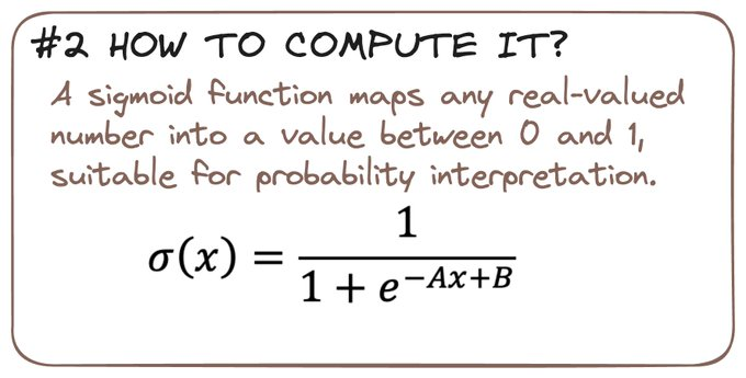
The Sigmoid Function is our mathematical wand, turning numbers into neat probabilities between 0 and 1.
It's what makes Logistic Regression tick, giving us a clear 'probabilistic' picture.
4
3️⃣ 𝗛𝗢𝗪 𝗧𝗢 𝗗𝗘𝗙𝗜𝗡𝗘 𝗧𝗛𝗘 𝗕𝗘𝗦𝗧 𝗙𝗜𝗧?
For every parametric ML algorithm, we need a LOSS FUNCTION.
It is our map to find our optimal solution or global minimum.
(hoping there is one! 😉)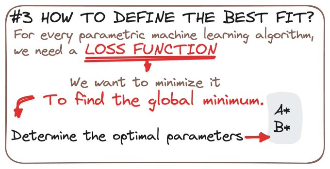
For every parametric ML algorithm, we need a LOSS FUNCTION.
It is our map to find our optimal solution or global minimum.
(hoping there is one! 😉)
5
✚ 𝗕𝗢𝗡𝗨𝗦 - FROM LINEAR TO LOGISTIC REGRESSION
To obtain the sigmoid function, we can derive it from the Linear Regression equation.
To obtain the sigmoid function, we can derive it from the Linear Regression equation.
6
4️⃣ 𝗛𝗢𝗪 𝗧𝗢 𝗢𝗕𝗧𝗔𝗜𝗡 𝗜𝗧 𝗠𝗔𝗧𝗛𝗘𝗠𝗔𝗧𝗜𝗖𝗔𝗟𝗟𝗬?
For a binary classification, the model output corresponds to a predicted y:
- 0 for one class
- 1 for the other one.
(Remember we are in a BINARY classification model... at least for now!)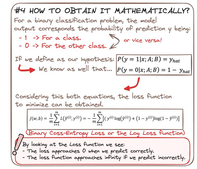
For a binary classification, the model output corresponds to a predicted y:
- 0 for one class
- 1 for the other one.
(Remember we are in a BINARY classification model... at least for now!)
7
𝗛𝗬𝗣𝗢𝗧𝗛𝗘𝗦𝗜𝗦
Assuming a hypothesis y_hat as the probability of y being 1, we get two main equations.
As a starting point, we mathematically obtain the corresponding LOSS FUNCTION from those equations.
We end up with the Binary Cross-Entropy or Log Loss Function.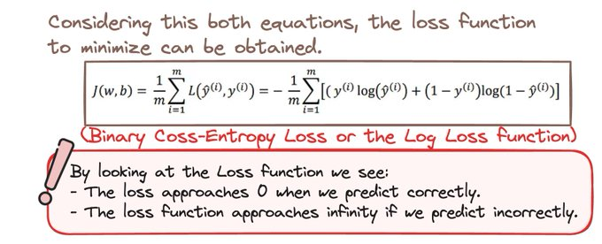
Assuming a hypothesis y_hat as the probability of y being 1, we get two main equations.
As a starting point, we mathematically obtain the corresponding LOSS FUNCTION from those equations.
We end up with the Binary Cross-Entropy or Log Loss Function.
8
5️⃣ 𝗙𝗜𝗡𝗗 𝗧𝗛𝗘 𝗢𝗣𝗧𝗜𝗠𝗔𝗟 𝗦𝗢𝗟𝗨𝗧𝗜𝗢𝗡
To find our optimal parameter values, we use the gradient descent.
It carefully navigates the cost function landscape, seeking the valley of optimal parameters.
And iteratively we get closer to the optimal solution.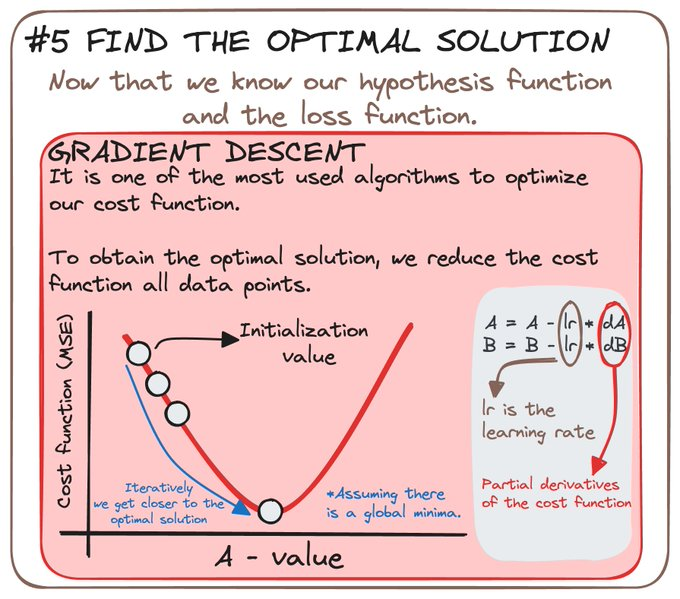
To find our optimal parameter values, we use the gradient descent.
It carefully navigates the cost function landscape, seeking the valley of optimal parameters.
And iteratively we get closer to the optimal solution.
9
6️⃣ 𝗠𝗢𝗗𝗘𝗟 𝗘𝗩𝗔𝗟𝗨𝗔𝗧𝗜𝗢𝗡
Once our model's journey is complete, we assess its valor through trials like the Confusion Matrix and ROC Curve.
Only the models that prove their worth will be knighted for deployment.
Once our model's journey is complete, we assess its valor through trials like the Confusion Matrix and ROC Curve.
Only the models that prove their worth will be knighted for deployment.
10
7️⃣ 𝗔𝗦𝗦𝗨𝗠𝗣𝗧𝗜𝗢𝗡𝗦 𝗢𝗙 𝗧𝗛𝗘 𝗠𝗢𝗗𝗘𝗟
Our Logistic Regression model is built on foundations firm in assumptions:
1. Binary outcomes.
2. Linearity in Log Odds.
3. No Multicollinearity
4. Large Sample Size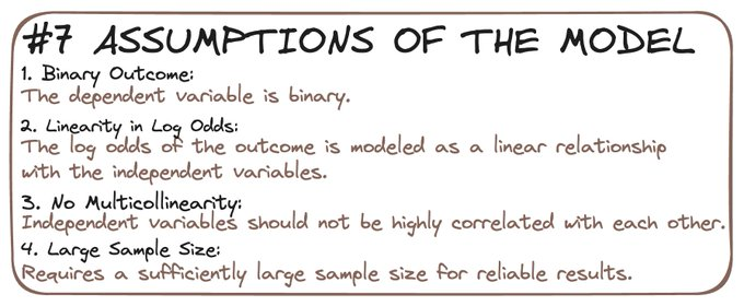
Our Logistic Regression model is built on foundations firm in assumptions:
1. Binary outcomes.
2. Linearity in Log Odds.
3. No Multicollinearity
4. Large Sample Size
11
Mastering Logistic Regression is a craft, a blend of art and science.
And this is all for now!
And this is all for now!
12
If you are interested in...
• Python 🐍
• SQL 💾
• ML/MLOps 🛠
• LLMs & NLP 🗣
• DataViz 🗣
• AI Engineering ⚙️
Then follow me → @rfeers
• Python 🐍
• SQL 💾
• ML/MLOps 🛠
• LLMs & NLP 🗣
• DataViz 🗣
• AI Engineering ⚙️
Then follow me → @rfeers
13
Did you like this thread?
Then join my DataBites newsletter to get all my content right to your mail every Sunday! 🧩
👉🏻 databites.tech 🤓
Then join my DataBites newsletter to get all my content right to your mail every Sunday! 🧩
👉🏻 databites.tech 🤓