
Every generate() call to an LLM runs two distinct computational phases on the same GPU:

• prefill (processing the prompt) is compute-bound
• while decode (generating tokens one at a time) is memory-bound.
Most inference optimizations target one phase or the other, and diagnosing which phase is the bottleneck is the first step in making a deployment faster.
In this article, I'll walk through the full pipeline, from tokenized input to streamed output, and look at where the time goes in each phase.
---
# Tokenization and embedding
Tokenizers like Byte Pair Encoding (BPE) convert raw text into integer IDs from a vocabulary of roughly 50,000 tokens.
prompt = "How does inference work?"
ids = tokenizer.encode(prompt)
# ids -> [2437, 1374, 32278, 670, 30]Each ID maps to a row in the embedding table, a learned matrix of shape [vocab_size, hidden_dim]. For a model with a hidden dimension of 4,096, each token becomes a 4,096-dimensional vector.
# embedding_table has shape [vocab_size, hidden_dim]
vectors = embedding_table[ids]   # shape: [num_tokens, 4096]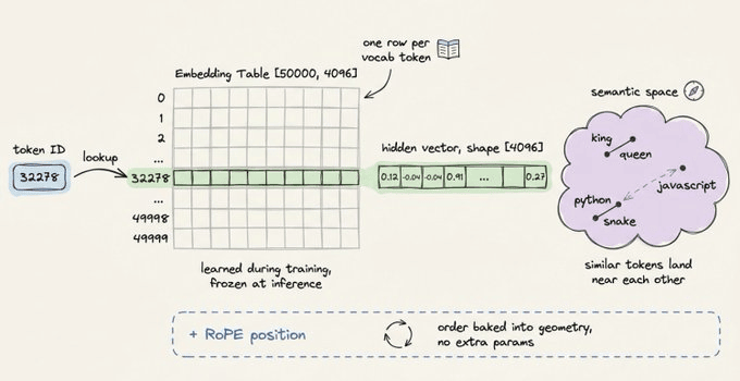
Position information gets injected at this stage.
Most modern architectures use Rotary Position Embeddings (RoPE), which encode position by rotating the embedding vectors rather than adding a separate positional vector.
---
# Transformer layers
The embedded sequence passes through a stack of transformer layers (typically 32 to 80+, depending on model size).
Each layer applies two operations in sequence:
1) Self-attention computes three projections per token (query Q, key K, value V) via learned weight matrices.

Generated by Thread Navigator
Press ⌘ + S to quick-export