How LLM Inference Works, Clearly Explained.
Every generate() call to an LLM runs two distinct computational phases on the same GPU:

Most inference optimizations target one phase or the other, and diagnosing which phase is the bottleneck is the first step in making a deployment faster.
In this article, I'll walk through the full pipeline, from tokenized input to streamed output, and look at where the time goes in each phase.
Tokenization and embedding
Tokenizers like Byte Pair Encoding (BPE) convert raw text into integer IDs from a vocabulary of roughly 50,000 tokens.
prompt = "How does inference work?"
ids = tokenizer.encode(prompt)
# ids -> [2437, 1374, 32278, 670, 30]
Each ID maps to a row in the embedding table, a learned matrix of shape [vocab_size, hidden_dim]. For a model with a hidden dimension of 4,096, each token becomes a 4,096-dimensional vector.
# embedding_table has shape [vocab_size, hidden_dim]
vectors = embedding_table[ids]   # shape: [num_tokens, 4096]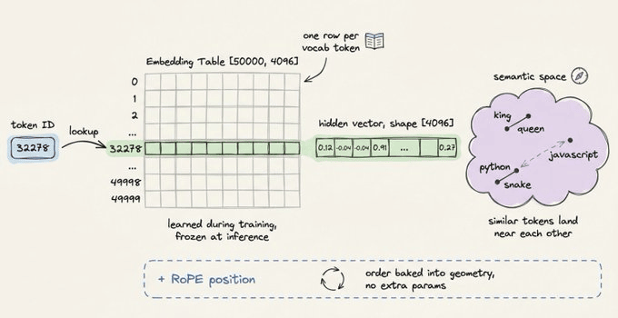
Position information gets injected at this stage.
Most modern architectures use Rotary Position Embeddings (RoPE), which encode position by rotating the embedding vectors rather than adding a separate positional vector.
Transformer layers
The embedded sequence passes through a stack of transformer layers (typically 32 to 80+, depending on model size).
Each layer applies two operations in sequence:
1) Self-attention computes three projections per token (query Q, key K, value V) via learned weight matrices.

Each token's query is scored against every other token's key, and those scores (after scaling and softmax) determine how much of each token's value gets mixed in.
# scores: how much each token attends to every other token
Q, K, V  = x @ Wq, x @ Wk, x @ Wv

scores = (Q @ K.T) / sqrt (d_k)

weights = softmax(scaled) # one row per token, sums to 1

attn_output  = weights @ V
2) Feed-forward network (FFN) processes each token's vector independently through a two-layer MLP. Attention moves information between positions. The FFN transforms it.
After the final layer, the model projects the last token's hidden state back to vocabulary size ([hidden_dim, vocab_size]), applies softmax, and samples from the resulting distribution to produce the first output token.
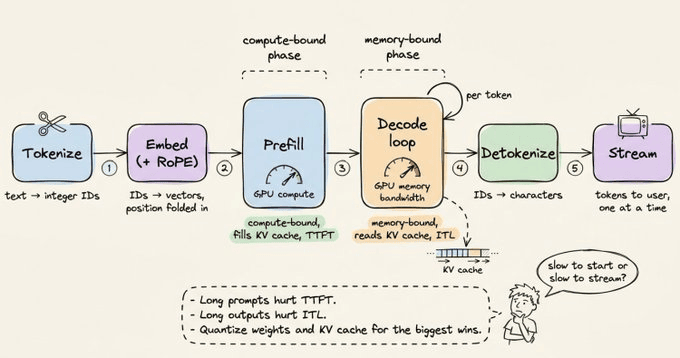
Prefill: the compute-bound phase
Processing the input prompt is the first phase. All tokens are processed in parallel: Q, K, and V are computed for every token simultaneously, and attention runs as a large matrix-matrix multiplication.
This is compute-bound work. The GPU's arithmetic throughput is the bottleneck, and utilization is high. The metric that captures this phase is Time to First Token (TTFT), the latency before the first output token appears.
During prefill, the model also populates the KV cache: the K and V tensors for every layer get stored in GPU memory for reuse.
# Prefill: process the whole prompt in one shot
hidden = embed(prompt_tokens) + positions
for layer in model.layers:
    Q, K, V = project(hidden)             # for ALL tokens at once
    hidden  = attention(Q, K, V) + hidden
    hidden  = feedforward(hidden) + hidden
    cache_kv(layer, K, V)                 # save for later
first_token = sample(project_to_vocab(hidden[-1]))
Decode: the memory-bound phase
Once the first token is generated, the model switches to generating one token at a time. For each new token, it only computes Q, K, and V for that single token. The K and V from all previous tokens are already in the cache.
# Decode: one token per iteration
token = first_token
steps = 0
while token != STOP and steps < MAX_STEPS:
    x = embed(token) + position(steps)
    for layer in model.layers:
        q, k, v = project(x)
        K_all, V_all = caches[layer].append(k, v) # cached history + new
        x = layer.forward(q, K_all, V_all, x)  # attention + FFN, residuals
    token = sample(project_to_vocab(x))
    steps += 1
    yield token
The arithmetic per step is tiny (one query vector against the cached key matrix instead of a full matrix-matrix multiply). But the GPU still loads every weight matrix and the entire cached K/V from memory for that small computation. The bottleneck flips from compute to memory bandwidth.

The metric for this phase is Inter-Token Latency (ITL): the time between consecutive output tokens. Low ITL is what makes a model feel responsive.
The KV cache
Without caching, generating a 1,000-token response would require recomputing attention over the entire growing sequence at every step, giving quadratic complexity.
The KV cache stores each layer's K and V tensors once and appends new entries incrementally.
The video below depicts LLM inference speed with vs. without KV caching:
The speedup is roughly 5x or more for long generations.
The cost is that the cache grows linearly with sequence length and exists per-layer. For a 13B-parameter model, the cache consumes roughly 1 MB per token. A 4K-token context burns through 4 GB of VRAM on the cache alone.
This is why long contexts get expensive. The cache competes directly with batch size for GPU memory, i.e., more cache per request means fewer concurrent requests per GPU.
Standard mitigations include quantizing the cache to INT8 or INT4, sliding window attention (dropping tokens outside a fixed window), grouped-query attention (GQA, sharing K/V across attention heads to reduce the number of cached tensors), and PagedAttention (the memory management trick behind vLLM that pages the cache like an OS pages virtual memory, eliminating fragmentation).
There's another interesting idea that I talked about around KV cache management below:
https://x.com/i/status/2070828078247604480
Redesigning attention around the cache
Quantization and paging treat the KV cache as a fixed cost to manage. DeepSeek's V4 series (released April 2025) takes a different approach: redesign attention so the cache is structurally smaller from the start.

V4 uses a hybrid of two compressed attention mechanisms.
Compressed Sparse Attention (CSA) compresses KV entries by 4x using softmax-gated pooling, then applies sparse attention over the compressed tokens.
Heavily Compressed Attention (HCA) is more aggressive. It consolidates KV entries across 128 tokens into a single compressed entry and applies dense attention over those representations.
At a 1M-token context, V4-Pro requires 27% of the single-token inference FLOPs and 10% of the KV cache compared to DeepSeek-V3.2.
In absolute terms, that's 9.62 GiB of KV cache per sequence at 1M context in bf16, compared to an estimated 83.9 GiB for a V3.2-style architecture. With fp4/fp8 quantization on top, the cache shrinks by another 2x.
The KV cache has become the constraint that the field is optimizing the model architecture around.
Quantization
Training uses FP32 or BF16 for gradient stability. Inference doesn't need that precision. The memory savings from reducing bit width are linear:

INT4 is why 7B models run on laptop GPUs with 4-6 GB of VRAM. Methods like GPTQ and AWQ use per-channel scaling factors to minimize quality degradation from the lossy compression.
Done well, INT4 lands within 1-2 percentage points of the full-precision model on standard benchmarks.
Going from FP16 to INT8 often cuts inference latency in half with negligible quality loss, making quantization the single highest-leverage optimization for most deployments.
Serving infrastructure
Modern inference servers wrap the prefill-decode loop with several optimizations:


I covered Speculative decoding in detail here:
https://x.com/i/status/2054860740541207032
Frameworks like vLLM, TensorRT-LLM, and Text Generation Inference (TGI) combine these techniques. A single GPU can serve dozens of concurrent users because decode leaves most of the arithmetic capacity idle, and continuous batching fills that idle capacity with other requests.
The full inference path
Some practical implications
When someone tells you their model is slow, the first diagnostic is whether it's slow to start (prefill-bound, optimize TTFT) or slow to stream (decode-bound, optimize ITL).
👉 Over to you: are you running into TTFT or ITL bottlenecks in your deployments, and what's worked for you?
That's a wrap!
If you enjoyed this tutorial:
Find me → @_avichawla
Every day, I share tutorials and insights on DS, ML, LLMs, and RAGs.