It's been a long time since I wrote anything remotely informative on X. I have something minor that sits somewhere in between [finance] signal analysis and statistics, which is also very practical, simple, and with a familiar ending. A loong 🧵 👇.
1/18

Say that you have excess independent asset returns📉📈, i.e., you have removed common components of returns so that your n-dimensional return vector z[t] has independent elements. Also, z-score them so that they have unit volatility. There are T investment epochs/year.
2/18
2/18
Your holy grail is to find a signal vector x[t], such that the cross-sectional correlation IC:=corr(x, z) is as high as possible (IC stands for "Information Coefficient"). Then the Sharpe Ratio is SR=IC*sqrt(n*T). Fundamental Law of Active Management. So far, so good.
3/18
3/18
However, say that you have a model in mind, where some asset-specific variables determine returns. Most common variable: EPS - baseline, were the baseline is consensus EPS, or something like it (because consensus is a bit too easy to beat!).
4/18
4/18
EPS is only one choice. The variable depends a lot on asset class, investment class, etc. It could be drug approval; or credit downgrade, etc. You get the idea. And there might be more than one (but we stick to one).
5/18
5/18
The important thing is: the variable, at some point, is observed. We can estimate the relationship variable-returns, after the it's been observed. You estimate IC_ideal := corr(y, z). If you choose the variable well, this correlation can be quite high. If you only knew y.
6/18
6/18
... you'd be rich. At least, you have a different problem: forecasting the variable y. You might like this problem, because you can encode a lot of expertise in the forecast. Say that you have forecasts x. The R^2 of the model y ~ x is Rsq. You'd like to use x as signals...
7/18
7/18
... as that is your best available information. You know that corr(x, y)=sqrt(Rsq). What you need is to know is the Sharpe Ratio of the strategy: corr(x, z)*sqrt(n).
8/18
8/18
The statistics part is this: if I know corr(x,y)=rho_1 and corr(y, z) = rho_2, what is corr(x, z)?
9/18
9/18
You have seen this at some point. A necessary condition for the correlation is that the determinant of the correlation matrix be positive definite.
10/18
10/18

From which we get a worst-case bound:
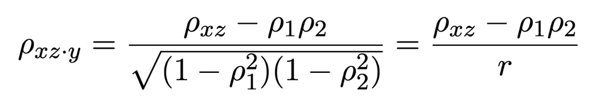
r:=sqrt[(1-rho_1^2)*(1-rho_2^2)] and
|rho_1*rho_2 - rho_xz| <= r. The problem is that they are usually not binding. A realistic example: rho_1=0.1, rho_2=0.6, then rho_1*rho_2=0.06 with a range of 0.8. Too wide!
11/18
r:=sqrt[(1-rho_1^2)*(1-rho_2^2)] and
|rho_1*rho_2 - rho_xz| <= r. The problem is that they are usually not binding. A realistic example: rho_1=0.1, rho_2=0.6, then rho_1*rho_2=0.06 with a range of 0.8. Too wide!
11/18
An alternative way to obtain the same bound (and more) is via partial correlation. The partial correlation of forecast and returns, given the realized variable, is below, and must be in [-1, 1].
12/18
12/18
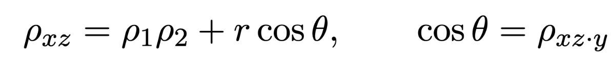
Geometrical view:
rho_xz = rho_1*rho_2 + r*cos(theta), with theta = cor(x, z|y)
for high n, it is reasonable to assume that partial correlation concentrates around 0. Given the realization of the variable, the forecast contains no information about the returns.
13/18
rho_xz = rho_1*rho_2 + r*cos(theta), with theta = cor(x, z|y)
for high n, it is reasonable to assume that partial correlation concentrates around 0. Given the realization of the variable, the forecast contains no information about the returns.
13/18
So we have an expectation identity: E[rho_xz]=rho_1*rho_2.
Now you can factor the Information Coefficient into the product of the sqrt(Rsq) of your forecast, and the IC_ideal, under knowledge of the key variables.
14/18
Now you can factor the Information Coefficient into the product of the sqrt(Rsq) of your forecast, and the IC_ideal, under knowledge of the key variables.
14/18
The annualized Sharpe Ratio is
Sharpe = sqrt(Rsq)*IC_ideal*sqrt(breath)*sqrt(# decisions/yr)
So there you have it.
15/18
Sharpe = sqrt(Rsq)*IC_ideal*sqrt(breath)*sqrt(# decisions/yr)
So there you have it.
15/18
Sharpe decompositions appear often in quantitative investment, but they have very different meanings. This one generalizes the Transfer Coefficient. Replace y with the *true* expected returns, x with the forecasts, and you get the TC identity in the Clarke et al. paper.
16/18
16/18
Last thing: I told the story with y as variables that predict returns from their historical realizations. But y and x can be anything. For example, y could be forecasts and x can be the noisy, corrupted estimates of these forecasts. Worst things can happen.
17/18
17/18
The story-time interpretation, though, is useful. We should use Oracles more, and then predict those Oracles, and combine them. People do this without thinking carefully about pitfalls and power-ups. Underrated and overrrated at the same time.
And that is the end.
18/18
And that is the end.
18/18
Generated by Thread Navigator
Press ⌘ + S to quick-export